10. Time Gating: Isolating Multipath and RIS Responses

What Is Time Gating?

Time gating is a signal-processing method that keeps or rejects a selected interval of a measured time-domain response. It is useful when several electromagnetic paths, reflections, connectors, antennas, or environmental scatterers contribute to one frequency-domain measurement.

Imagine hearing one hand clap in a room. The first arrival may be the direct sound, followed by echoes from different walls. A time gate is like selecting only the short interval containing one chosen echo. In an RF measurement, the selected object is usually a complex impulse response rather than an audible waveform.

The basic processing chain is

Time gating does not physically remove a reflector from the room. It produces a processed response in which contributions outside the chosen delay interval are attenuated.

References for this section3

• Y. Ren et al., "Time-Domain Channel Measurements and Small-Scale Fading Characterization for RIS-Assisted Wireless Communication Systems", IEEE Transactions on Vehicular Technology, vol. 73, no. 10, pp. 14127–14142, 2024.
• Keysight Technologies, "Time Domain", VNA help documentation covering transforms, resolution, alias-free range, windows, and gating.
• Keysight Technologies, "Time Domain Analysis Using a Network Analyzer", Application Note 1287-12.

Why and Where Is It Used?

Common applications include:

• separating antenna reflections from chamber, floor, wall, cable, or fixture reflections;
• locating faults and impedance discontinuities along cables;
• removing connector or adapter responses from VNA measurements;
• isolating one path in a wideband wireless channel;
• estimating power-delay profiles, path delays, path powers, and delay spread;
• selecting the RIS-assisted path while suppressing direct leakage and unrelated multipath;
• transforming the isolated path back to frequency to examine its magnitude and phase versus frequency.

A gate can be band-pass in time, which keeps responses inside the interval, or notch in time, which rejects responses inside the interval.

References for this section3

• Y. Ren et al., "Time-Domain Channel Measurements and Small-Scale Fading Characterization for RIS-Assisted Wireless Communication Systems", IEEE Transactions on Vehicular Technology, vol. 73, no. 10, pp. 14127–14142, 2024.
• D. M. Pozar, Microwave Engineering, 4th ed., Wiley, 2012.
• Rohde & Schwarz, "Time Domain Measurements Using Vector Network Analyzer ZNA", Application Note 1EP83, 2020.

The Multipath Channel Model

For a static narrow observation period, a multipath channel can be represented as

$$h(\tau) = \sum_{\ell=0}^{L-1} \alpha_{\ell} e^{j\psi_{\ell}} \delta(\tau-\tau_{\ell}),$$

where

• $\alpha_{\ell}$ is the amplitude of path $\ell$;
• $\psi_{\ell}$ is its phase;
• $\tau_{\ell}$ is its propagation delay;
• $\delta(\cdot)$ represents an ideal impulse at that delay.

The corresponding frequency response is the Fourier transform of the impulse response:

$$H(f) = \int_{-\infty}^{\infty} h(\tau)e^{-j2\pi f\tau}\,d\tau = \sum_{\ell=0}^{L-1} \alpha_{\ell}e^{j\psi_{\ell}}e^{-j2\pi f\tau_{\ell}}.$$

Every path therefore produces a phase slope versus frequency. A longer delay gives a faster phase rotation with frequency.

References for this section3

• Y. Ren et al., "Time-Domain Channel Measurements and Small-Scale Fading Characterization for RIS-Assisted Wireless Communication Systems", IEEE Transactions on Vehicular Technology, vol. 73, no. 10, pp. 14127–14142, 2024.
• D. M. Pozar, Microwave Engineering, 4th ed., Wiley, 2012.
• Keysight Technologies, "Time Domain Analysis Using a Network Analyzer", Application Note 1287-12.

From Measured Frequency Samples to Delay

Suppose a VNA or channel sounder measures $N$ complex samples

$$H[k]=H(f_0+k\Delta f), \qquad k=0,1,\ldots,N-1.$$

After applying a frequency-domain window $W[k]$, the discrete delay response is calculated with an inverse discrete Fourier transform:

$$\widetilde{h}[m] = \frac{1}{N} \sum_{k=0}^{N-1} W[k]H[k] e^{j2\pi km/N}.$$

In software this is normally evaluated using an IFFT. The measured power-delay profile is then proportional to

$$P[m]=|\widetilde{h}[m]|^2.$$

Peaks in $P[m]$ indicate strong arrivals at different delays. They may correspond to a direct path, an RIS route, a wall reflection, or another scattering cluster.

References for this section3

• Y. Ren et al., "Time-Domain Channel Measurements and Small-Scale Fading Characterization for RIS-Assisted Wireless Communication Systems", IEEE Transactions on Vehicular Technology, vol. 73, no. 10, pp. 14127–14142, 2024.
• D. M. Pozar, Microwave Engineering, 4th ed., Wiley, 2012.
• Keysight Technologies, "Time Domain Analysis Using a Network Analyzer", Application Note 1287-12.

Is a Fourier Series Required?

No separate Fourier-series derivation is normally required.

A Fourier series describes a periodic signal as a sum of harmonically related sinusoids. Time gating of measured RF channel data normally uses the Fourier transform or its sampled implementation, the DFT/FFT and IDFT/IFFT. The operations are related mathematically, but the practical workflow is:

1. acquire complex frequency samples;
2. use an IFFT to obtain the delay-domain response;
3. multiply by a time gate;
4. use an FFT if a gated frequency response is required.

The complex phase must be retained. Transforming only frequency-domain magnitude discards the phase information needed to place responses correctly in delay.

References for this section3

• Y. Ren et al., "Time-Domain Channel Measurements and Small-Scale Fading Characterization for RIS-Assisted Wireless Communication Systems", IEEE Transactions on Vehicular Technology, vol. 73, no. 10, pp. 14127–14142, 2024.
• D. M. Pozar, Microwave Engineering, 4th ed., Wiley, 2012.
• Keysight Technologies, "Time Domain", VNA help documentation covering transforms, resolution, alias-free range, windows, and gating.

How the Gate Works Mathematically

Let $g(\tau)$ be a gate centred on the desired arrival. The gated response is

$$h_{\mathrm{g}}(\tau) = g(\tau)h(\tau).$$

For an ideal rectangular gate from $\tau_1$ to $\tau_2$,

$$g(\tau) = \begin{cases} 1, & \tau_1\leq\tau\leq\tau_2,\\ 0, & \text{otherwise}. \end{cases}$$

If the selected peak belongs to path $p$ and the other resolved paths fall outside the interval, then

$$h_{\mathrm{g}}(\tau) \approx \alpha_p e^{j\psi_p}\delta(\tau-\tau_p).$$

Transforming back gives the path-isolated frequency response

$$H_{\mathrm{g}}(f) = \mathcal{F}\{h_{\mathrm{g}}(\tau)\}.$$

Multiplication in time corresponds to convolution in frequency:

$$H_{\mathrm{g}}(f) = H(f)*G(f).$$

This is why an abrupt rectangular gate can create frequency-domain ripple. Smooth gates such as Hann, Tukey, or Kaiser windows reduce sidelobes, but broaden the selected response. Gate design is therefore a trade-off between delay resolution, leakage, and frequency-domain distortion.

References for this section3

• Y. Ren et al., "Time-Domain Channel Measurements and Small-Scale Fading Characterization for RIS-Assisted Wireless Communication Systems", IEEE Transactions on Vehicular Technology, vol. 73, no. 10, pp. 14127–14142, 2024.
• D. M. Pozar, Microwave Engineering, 4th ed., Wiley, 2012.
• Keysight Technologies, "Time Domain", VNA help documentation covering transforms, resolution, alias-free range, windows, and gating.

Can Time Gating Separate Multipath?

Yes—when the paths are sufficiently separated in delay and the measurement has enough bandwidth.

For a swept bandwidth $B$, a useful first-order delay-resolution rule is

$$\Delta\tau_{\mathrm{res}} \approx \frac{1}{B}.$$

Two paths with

$$|\tau_1-\tau_2| \gg \Delta\tau_{\mathrm{res}}$$

can normally be distinguished more easily. Actual resolution depends on the transform mode and window. A stronger smoothing window lowers sidelobes but widens each peak.

The frequency spacing determines the alias-free delay span:

$$T_{\mathrm{max}} \approx \frac{1}{\Delta f}.$$

For a transmission channel, a delay corresponds to total propagation length

$$D=c\tau$$

in free space. For a one-port reflection measurement, the wave travels outward and back, so the physical reflector distance is approximately

$$D_{\mathrm{reflection}} = \frac{c\tau}{2}.$$

Time gating cannot separate two paths whose peaks overlap inside the available delay resolution. It also cannot reconstruct energy that an earlier physical discontinuity prevented from reaching a later one.

References for this section3

• Keysight Technologies, "Time Domain", VNA help documentation covering transforms, resolution, alias-free range, windows, and gating.
• Y. Ren et al., "Time-Domain Channel Measurements and Small-Scale Fading Characterization for RIS-Assisted Wireless Communication Systems", IEEE Transactions on Vehicular Technology, vol. 73, no. 10, pp. 14127–14142, 2024.
• D. M. Pozar, Microwave Engineering, 4th ed., Wiley, 2012.

RIS-Assisted Communication Example

Consider a wideband transmission measurement with three main routes:

1. weak direct leakage with total length $7\ \mathrm{m}$;
2. the intended Tx–RIS–UE route with $d_{\mathrm{TR}}=4\ \mathrm{m}$ and $d_{\mathrm{RU}}=6\ \mathrm{m}$;
3. an environmental wall route with total length $13\ \mathrm{m}$.

Their approximate free-space delays are

$$\begin{aligned} \tau_{\mathrm{direct}}&=\frac{7}{c}=23.3\ \mathrm{ns},\\ \tau_{\mathrm{RIS}}&=\frac{4+6}{c}=33.3\ \mathrm{ns},\\ \tau_{\mathrm{wall}}&=\frac{13}{c}=43.3\ \mathrm{ns}. \end{aligned}$$

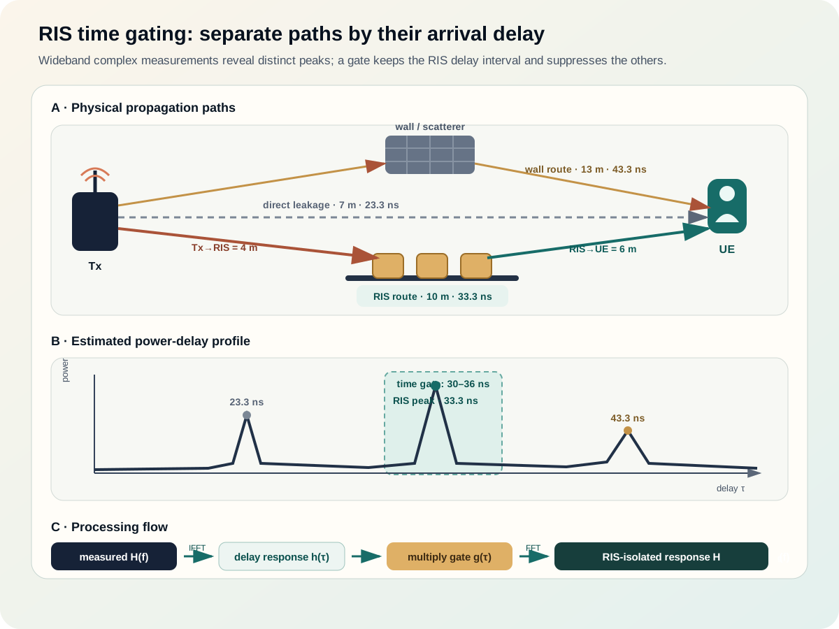
With $B=1\ \mathrm{GHz}$, the ideal first-order delay resolution is approximately

$$\Delta\tau_{\mathrm{res}} \approx \frac{1}{10^9} =1\ \mathrm{ns}.$$

The arrivals in this example are separated by about $10\ \mathrm{ns}$, so they are resolvable in principle. A gate spanning approximately $30$–$36\ \mathrm{ns}$ can isolate the RIS peak while allowing transition width around it.

The RIS-isolated response can then be written as

$$h_{\mathrm{RIS}}(\tau) = g_{\mathrm{RIS}}(\tau)h(\tau),$$

and transformed back to

$$H_{\mathrm{RIS}}(f) = \mathcal{F}\{h_{\mathrm{RIS}}(\tau)\}.$$

This allows the RIS path's frequency-dependent magnitude, phase, group delay, and path gain to be studied without most delay-resolved environmental contributions.

References for this section3

• Y. Ren et al., "Time-Domain Channel Measurements and Small-Scale Fading Characterization for RIS-Assisted Wireless Communication Systems", IEEE Transactions on Vehicular Technology, vol. 73, no. 10, pp. 14127–14142, 2024.
• Keysight Technologies, "Time Domain", VNA help documentation covering transforms, resolution, alias-free range, windows, and gating.
• D. M. Pozar, Microwave Engineering, 4th ed., Wiley, 2012.

A Stronger RIS Measurement Procedure

Time gating becomes more reliable when combined with controlled RIS states.

Measure the complex channel with the RIS configured toward the UE:

$$H_{\mathrm{on}}(f) = H_{\mathrm{static}}(f) +H_{\mathrm{RIS,on}}(f).$$

Then measure a reference state, such as an absorption-like state, randomized state, or a configuration that directs energy away from the UE:

$$H_{\mathrm{ref}}(f) = H_{\mathrm{static}}(f) +H_{\mathrm{RIS,ref}}(f).$$

Complex subtraction gives

$$\Delta H(f) = H_{\mathrm{on}}(f)-H_{\mathrm{ref}}(f),$$

which suppresses static components that remain unchanged between the two measurements. Then compute

$$\Delta h(\tau) = \mathcal{F}^{-1}\{W(f)\Delta H(f)\}$$

and gate around the predicted RIS delay

$$\tau_{\mathrm{RIS}} = \frac{d_{\mathrm{TR}}+d_{\mathrm{RU}}}{c}.$$

This state differencing plus time gating is often more convincing than selecting a peak only because it appears near the expected delay. The reference and active measurements must remain phase coherent; movement, oscillator drift, or timing changes between sweeps can spoil the subtraction.

References for this section3

• Y. Ren et al., "Time-Domain Channel Measurements and Small-Scale Fading Characterization for RIS-Assisted Wireless Communication Systems", IEEE Transactions on Vehicular Technology, vol. 73, no. 10, pp. 14127–14142, 2024.
• D. M. Pozar, Microwave Engineering, 4th ed., Wiley, 2012.
• Keysight Technologies, "Time Domain", VNA help documentation covering transforms, resolution, alias-free range, windows, and gating.

Step-by-Step Workflow

1. Choose bandwidth and frequency step. Ensure the bandwidth can resolve the expected path-delay differences and the frequency step provides enough alias-free delay range.
2. Calibrate the reference planes. Remove systematic cable, connector, and instrument errors before interpreting delay.
3. Measure complex data. Record both magnitude and phase of $S_{21}(f)$ or the channel transfer function.
4. Apply a frequency window. Select the resolution-versus-sidelobe trade-off deliberately.
5. Compute the IFFT. Form the complex impulse response and power-delay profile.
6. Predict the desired delay. Use geometry, ray tracing, or a marker measurement to estimate the Tx–RIS–UE delay.
7. Place a smooth gate. Include the complete desired peak and its main lobe without admitting neighbouring paths.
8. Check stability. Change gate width and window slightly; a physical conclusion should not depend on one arbitrary boundary.
9. Transform back if needed. Use an FFT to recover the gated frequency response.
10. Report processing choices. State frequency span, point count, window, gate centre, gate width, calibration plane, and whether state subtraction was used.

References for this section3

• Y. Ren et al., "Time-Domain Channel Measurements and Small-Scale Fading Characterization for RIS-Assisted Wireless Communication Systems", IEEE Transactions on Vehicular Technology, vol. 73, no. 10, pp. 14127–14142, 2024.
• D. M. Pozar, Microwave Engineering, 4th ed., Wiley, 2012.
• Keysight Technologies, "Time Domain", VNA help documentation covering transforms, resolution, alias-free range, windows, and gating.

What Time Gating Can and Cannot Prove

Time gating can show that measurable energy exists near a predicted delay and can isolate that delay-resolved component. It can support path attribution when combined with geometry, RIS state changes, angular measurements, or controlled blockage.

Time gating alone does not prove that a peak came from the RIS. Different paths can share similar delay, peaks can overlap, and finite bandwidth produces sidelobes. Stronger evidence comes from repeating the measurement across RIS states and showing that the selected component changes according to the programmed RIS response while static environmental paths remain comparatively stable.

References for this section3

• Y. Ren et al., "Time-Domain Channel Measurements and Small-Scale Fading Characterization for RIS-Assisted Wireless Communication Systems", IEEE Transactions on Vehicular Technology, vol. 73, no. 10, pp. 14127–14142, 2024.
• Keysight Technologies, "Time Domain", VNA help documentation covering transforms, resolution, alias-free range, windows, and gating.
• Rohde & Schwarz, "Time Domain Measurements Using Vector Network Analyzer ZNA", Application Note 1EP83, 2020.

Practical Interpretation

• A larger peak in the gated RIS interval indicates more energy at that delay, not automatically better end-to-end data rate.
• Reduced RMS delay spread can reduce frequency selectivity, but the result depends on the complete channel and receiver bandwidth.
• A very narrow rectangular gate may look selective while producing substantial frequency ripple.
• A very wide gate may preserve the waveform but also admit unwanted multipath.
• More bandwidth improves delay resolution; more closely spaced frequency samples increase the observable delay range.
• Dynamic channels require fast or synchronized acquisition because moving objects change path delay and phase during the sweep.

References for this section3

• Y. Ren et al., "Time-Domain Channel Measurements and Small-Scale Fading Characterization for RIS-Assisted Wireless Communication Systems", IEEE Transactions on Vehicular Technology, vol. 73, no. 10, pp. 14127–14142, 2024.
• D. M. Pozar, Microwave Engineering, 4th ed., Wiley, 2012.
• Keysight Technologies, "Time Domain", VNA help documentation covering transforms, resolution, alias-free range, windows, and gating.

Takeaway

Time gating converts a complex wideband measurement into delay, selects the interval containing a desired response, and optionally transforms that response back to frequency. It can separate multipath only when the measurement bandwidth resolves the arrivals. In RIS-assisted experiments, the most defensible workflow combines predicted Tx–RIS–UE delay, complex RIS-state differencing, a documented smooth gate, and sensitivity checks on the window and gate width.

References for this section3

• Y. Ren et al., "Time-Domain Channel Measurements and Small-Scale Fading Characterization for RIS-Assisted Wireless Communication Systems", IEEE Transactions on Vehicular Technology, vol. 73, no. 10, pp. 14127–14142, 2024.
• D. M. Pozar, Microwave Engineering, 4th ed., Wiley, 2012.
• Keysight Technologies, "Time Domain", VNA help documentation covering transforms, resolution, alias-free range, windows, and gating.