3. Signal Processing Performance: What to Measure

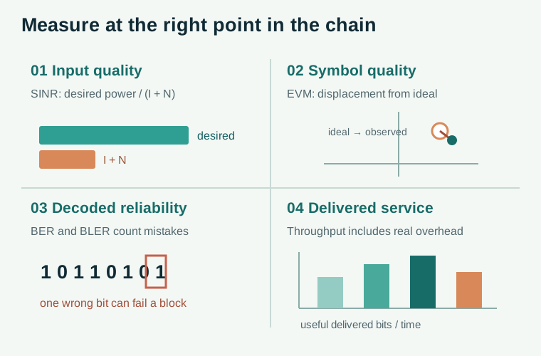
Choose a Metric for the Question

A clean-looking spectrum does not guarantee correct decoded bits. Measure the physical input and the delivered result.

• Input: power, noise, interference, and channel conditions.
• Inside the receiver: channel estimate and constellation displacement.
• Outcome: wrong bits or blocks, delivered throughput, and latency.
• No universal target: EVM, BER, and SINR limits depend on modulation, coding, bandwidth, channel, and service.

Metric	Physical meaning	Use it when
SNR / SINR	Desired signal relative to noise / noise plus interference	Describing the receiver's available signal quality
EVM	RMS distance of recovered constellation points from ideal references	Diagnosing modulation quality, distortion, and residual receiver errors
Channel-estimation MSE / NMSE	Difference between estimated and known channel, optionally normalized	Comparing estimators in simulation or controlled measurement
BER / BLER	Fraction of wrong bits / failed decoded blocks	Judging data reliability after specified receiver stages
Throughput / spectral efficiency	Delivered data per second / per second per hertz	Assessing useful capacity including overhead and retransmissions
PAPR	Peak waveform power relative to average power	Checking OFDM amplifier back-off and clipping risk
Processing latency and complexity	Time and resources needed to produce a result	Checking real-time and implementation feasibility
Localization MAE / RMSE	Typical absolute or squared-error-weighted position difference	Comparing location estimators on the same test positions

• EVM: how far measured constellation points move from their ideal positions.
• BER: fraction of wrong bits at a named processing stage.
• BLER: fraction of failed decoded blocks.
• Important: EVM is not BER; state the measurement point, reference, and normalization.

For reference constellation symbols $s_i$ and measured symbols $\widehat s_i$, one common RMS definition is

$$\mathrm{EVM}_{\mathrm{RMS}}= 100\sqrt{\frac{\sum_i|\widehat s_i-s_i|^2}{\sum_i|s_i|^2}}\ \%$$

• $\mathrm{EVM}_{\mathrm{RMS}}$: RMS error vector magnitude as a percentage under this normalization.
• $s_i$: ideal reference symbol $i$; $\widehat s_i$: measured symbol at the same position.
• $i$: index over measured symbols; $|\cdot|$ gives complex-vector magnitude.
• Comparison: instrument reference, equalization, and normalization settings must match.

For a test with known transmitted bits and blocks,

$$\mathrm{BER}=\frac{N_{\mathrm{wrong\ bits}}}{N_{\mathrm{tested\ bits}}}, \qquad \mathrm{BLER}=\frac{N_{\mathrm{failed\ blocks}}}{N_{\mathrm{tested\ blocks}}}$$

• $N_{\mathrm{wrong\ bits}}$, $N_{\mathrm{tested\ bits}}$: bit mismatches and total checked bits.
• $N_{\mathrm{failed\ blocks}}$, $N_{\mathrm{tested\ blocks}}$: failed decoded blocks and total checked blocks.
• Observation length: zero errors in a short test does not prove zero true error probability.

References for this section3

• MathWorks, Measure Modulation Accuracy.
• MathWorks, Bit Error Rate Analysis Techniques.
• MathWorks, Communications Toolbox Test and Measurement.

Worked Example: Follow One Test Through the Chain

Imagine a controlled 10 MHz link and follow it through four measurement points:

1. Constellation: RMS error is 0.1 times reference RMS amplitude; EVM is 10% under the equation above.
2. Decoded bits: 7 of 10,000 test bits differ; BER is $7/10000=7\times10^{-4}$.
3. Decoded blocks: 2 of 100 blocks fail; BLER is 2%.
4. Delivered service: 10 Mbit of useful data arrive in 2 seconds; throughput is 5 Mbit/s and delivered spectral efficiency is $5/10=0.5$ bit/s/Hz.

These are distinct measurements; one generally cannot be calculated from another without more assumptions.

References for this section3

• MathWorks, Measure Modulation Accuracy.
• MathWorks, Bit Error Rate Analysis Techniques.
• MathWorks, Communications Toolbox Test and Measurement.

Additional Parameters for Specific Tasks

PAPR compares the largest OFDM waveform power with its average power:

$$\mathrm{PAPR}=\frac{\max_n|x[n]|^2}{\frac{1}{N}\sum_{n=0}^{N-1}|x[n]|^2}$$

• $x[n]$: complex time-domain sample; $n$ indexes samples and $N$ is the observation length.
• $\max_n|x[n]|^2$: peak sample power; the denominator is average sample power.
• Physical meaning: high peaks need amplifier headroom; clipping can worsen EVM and out-of-band emissions.
• Measure: report a distribution over many symbols, not one convenient block.

For channel estimation, normalized MSE is often

$$\mathrm{NMSE}=\frac{\sum\|\widehat H-H\|^2}{\sum\|H\|^2}$$

• $H$: trusted true channel; $\widehat H$: estimated channel.
• $\|\cdot\|^2$: squared error or energy over the chosen dimensions.
• $\sum$: sum over the stated antennas, subcarriers, times, or locations.
• Caution: ground truth is easy in simulation but difficult in a field measurement.

For localization, measure each position's distance error $e_i$:

$$\mathrm{MAE}=\frac{1}{N}\sum_{i=1}^{N}|e_i|,\qquad \mathrm{RMSE}=\sqrt{\frac{1}{N}\sum_{i=1}^{N}e_i^2}$$

• $e_i$: position-error distance for test point $i$, in metres; $N$ is the number of test points.
• MAE: average error magnitude; RMSE: penalizes large misses more strongly.
• Example: errors of 1 m, 1 m, and 10 m give MAE 4 m and RMSE about 5.83 m.
• Also report: median and 90th percentile, so occasional large misses remain visible.

References for this section3

• MathWorks, Measure Modulation Accuracy.
• MathWorks, Bit Error Rate Analysis Techniques.
• MathWorks, Communications Toolbox Test and Measurement.

Read Results in the Right Order

1. Fix the comparison: same waveform, bandwidth, channel realizations, antenna setup, transmit power, and receiver assumptions.
2. Inspect received power and SINR to describe the physical input, then synchronization and channel-estimation error to locate processing problems.
3. Compare EVM at the constellation with BER/BLER after decoding. If they disagree, inspect coding, retransmissions, and measurement points.
4. Report throughput or spectral efficiency only after including pilot, prefix, control, and retransmission overhead as appropriate.
5. For localization, report error distribution or percentile alongside MAE/RMSE, and separate training locations from test locations.

• Lower NMSE but same BLER: the decoder may already tolerate the original estimation error.
• Low mean position error: can hide severe misses; show a percentile or error CDF.
• Fair claim: keep baseline and test conditions comparable.

References for this section3

• MathWorks, Measure Modulation Accuracy.
• MathWorks, Bit Error Rate Analysis Techniques.
• MathWorks, Communications Toolbox Test and Measurement.

Application: Choose the Right Plot

• Coverage claim: show RSRP or received-power distribution, SINR distribution, and outage at a declared threshold.

• Receiver algorithm claim: show BER/BLER versus SNR or $E_b/N_0$, plus complexity and latency under the same channel seeds.

• Beamforming claim: show desired-user SINR, interference leakage, and performance over steering angle; specify total-power normalization.

• Localization claim: show the error CDF and spatial error map, not only a single mean; test on positions unseen during tuning.

• Baseline: compare with a simple established method.

• Same conditions: fix train/test split, channel, power, and waveform.

• Uncertainty and cost: report variation across runs and resources needed for the gain.

• Cellular readings: RSSI, RSRP, SNR, SINR, and CQI.

• Physical cause: propagation basics.

References for this section3

• MathWorks, Measure Modulation Accuracy.
• MathWorks, Bit Error Rate Analysis Techniques.
• MathWorks, Communications Toolbox Test and Measurement.