2. Propagation: What the Channel Does

Start With One Street-Corner Link

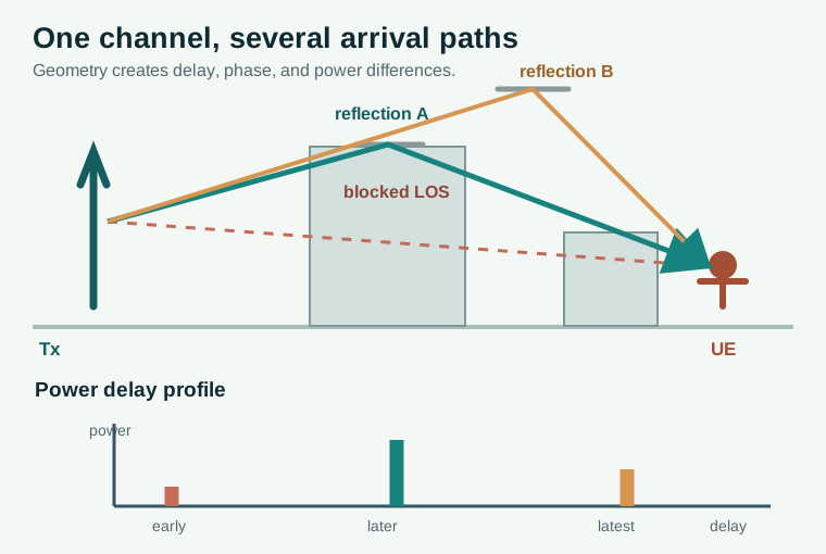
A receiver hears one direct wave and later echoes from buildings. Each arrival can have a different strength, delay, direction, and phase.

• Channel: the combined effect of those paths on the transmitted signal.
• Reflection: a path bounces off a surface; diffraction: it bends around an edge; shadowing: a large object weakens important paths.
• Why it matters: a strong average signal can still fade when the paths cancel at a particular location or frequency.

References for this section3

• 3GPP, TR 38.901: Study on channel model for frequencies from 0.5 to 100 GHz.
• ITU-R, Recommendation P.525-5: Calculation of free-space attenuation.
• MathWorks, Transmission Over MIMO Channel Model with Delay Profile TDL.

Path Loss and Shadowing

Path loss is the average power reduction between transmitter and receiver. Shadowing is the slower extra change caused by large obstructions.

• Physical view: distance reduces the available power; a wall or vehicle may remove the direct path.
• Use: estimate coverage and the extra link margin needed for blocked positions.
• Keep separate: antenna gain, feed loss, polarization loss, and propagation loss should not be counted twice.

For an ideal unobstructed far-field reference with isotropic antennas:

$$L_{\mathrm{FS,dB}}=20\log_{10}\!\left(\frac{4\pi d}{\lambda}\right)$$

• $L_{\mathrm{FS,dB}}$: free-space path loss in dB.
• $d$: transmitter-to-receiver distance in metres.
• $\lambda$: wavelength in metres; $\lambda=c/f$ for frequency $f$ and wave speed $c$.
• $\pi$: the usual mathematical constant; the logarithm converts a power ratio into decibels.

Example: at 28 GHz and 100 m, $\lambda\approx0.0107$ m and free-space loss is about 101.4 dB. Doubling distance adds about 6 dB only in this ideal reference. Street geometry can change the measured slope.

References for this section3

• ITU-R, Recommendation P.525-5: Calculation of free-space attenuation.
• 3GPP, TR 38.901: Study on channel model for frequencies from 0.5 to 100 GHz.
• NIST, Millimeter-Wave Channel Sounding and Modeling.

Delay and Excess Delay

Delay is the travel time of one path. Excess delay compares an arrival with the first detected arrival, so the first has zero excess delay.

• Direct path: often arrives first, but it may be blocked or too weak to detect.
• Later reflection: travels farther and arrives later; it can still be stronger than the first detected path.
• Use: estimate timing error and whether echoes overlap neighbouring symbols.

$$\tau_{\ell,\mathrm{excess}}=\tau_\ell-\tau_{\mathrm{first}}$$

• $\tau_\ell$: absolute arrival delay of path $\ell$.
• $\tau_{\mathrm{first}}$: delay of the first detected path, using the same clock.
• $\tau_{\ell,\mathrm{excess}}$: extra delay of path $\ell$, usually reported in ns or $\mu$s.

Example: arrivals at 330 ns and 430 ns have excess delays of 0 and 100 ns. Excess delay does not reveal where the reflector is without more geometry.

References for this section3

• ITU-R, Recommendation P.525-5: Calculation of free-space attenuation.
• 3GPP, TR 38.901: Study on channel model for frequencies from 0.5 to 100 GHz.
• MathWorks, Transmission Over MIMO Channel Model with Delay Profile TDL.

Power Delay Profile (PDP)

A PDP plots received path power against excess delay. Read its horizontal axis as when the echo arrives, and its vertical axis as how strong that echo is.

• Tap: one resolved delay bin or modeled path; a measured tap can contain several unresolved rays.
• Peak: a strong arrival, not necessarily the direct path.
• Use: see whether significant echoes fit inside an OFDM cyclic prefix and assess frequency selectivity.

For an idealized discrete-path channel:

$$h(t,\tau)=\sum_{\ell=1}^{L}a_\ell(t)\,\delta\!\left(\tau-\tau_\ell(t)\right)$$

• $h(t,\tau)$: channel impulse response at observation time $t$ and path delay $\tau$.
• $L$ and $\ell$: number of modeled paths and the path index.
• $a_\ell(t)$: complex path amplitude; its magnitude gives strength and its angle gives phase.
• $\tau_\ell(t)$: arrival delay of path $\ell$; $\delta$ marks an idealized arrival at that delay.

At a fixed observation time, the idealized PDP can be written as:

$$P(\tau)=\sum_{\ell=1}^{L}P_\ell\,\delta(\tau-\tau_{\ell,\mathrm{excess}}),\qquad P_\ell=|a_\ell|^2$$

• $P(\tau)$: power associated with each excess-delay location.
• $P_\ell$: linear power of path $\ell$; do not add dBm values directly.
• $a_\ell$, $L$, $\ell$, $\delta$, and $\tau_{\ell,\mathrm{excess}}$: path amplitude, count, index, idealized impulse, and excess delay defined above.

References for this section3

• MathWorks, Transmission Over MIMO Channel Model with Delay Profile TDL.
• 3GPP, TR 38.901: Study on channel model for frequencies from 0.5 to 100 GHz.
• ITU-R, Recommendation P.525-5: Calculation of free-space attenuation.

Mean Delay and RMS Delay Spread

Mean excess delay is the power-weighted centre of the PDP. RMS delay spread says how widely the significant arrivals sit around that centre.

$$\bar\tau=\frac{\sum_{\ell=1}^{L}P_\ell\tau_{\ell,\mathrm{excess}}}{\sum_{\ell=1}^{L}P_\ell}$$

• $\bar\tau$: mean excess delay, in seconds.
• $P_\ell$: linear power of path $\ell$; stronger paths carry more weight.
• $\tau_{\ell,\mathrm{excess}}$: excess delay of path $\ell$; $L$ is the number of paths.

$$\sigma_\tau=\sqrt{\frac{\sum_{\ell=1}^{L}P_\ell(\tau_{\ell,\mathrm{excess}}-\bar\tau)^2}{\sum_{\ell=1}^{L}P_\ell}}$$

• $\sigma_\tau$: RMS delay spread, in seconds; larger values mean more time dispersion.

• $P_\ell$, $\tau_{\ell,\mathrm{excess}}$, $\bar\tau$, and $L$: path power, excess delay, mean delay, and path count from the preceding equation.

• Example: two equally strong arrivals at 0 and 100 ns give mean delay 50 ns and RMS delay spread 50 ns.

• Consequence: large spread can cause frequency-selective fading and inter-symbol interference.

• Caution: coherence bandwidth is an approximate inverse-scale summary, not a universal fixed constant.

References for this section3

• ITU-R, Recommendation P.525-5: Calculation of free-space attenuation.
• 3GPP, TR 38.901: Study on channel model for frequencies from 0.5 to 100 GHz.
• MathWorks, Transmission Over MIMO Channel Model with Delay Profile TDL.

Doppler Shift and Doppler Spread

Doppler shift is a frequency change caused by motion along one path. Doppler spread describes the range of shifts across paths arriving from different directions.

$$f_{D,\ell}=\frac{v}{\lambda}\cos\theta_\ell$$

• $f_{D,\ell}$: signed Doppler shift of path $\ell$ in hertz; sign depends on the chosen direction convention.

• $v$: receiver speed in metres per second relative to the path geometry.

• $\lambda$: wavelength in metres; $\theta_\ell$ is the angle between movement and the path direction.

• Physical view: motion toward a path compresses the received wave cycles; motion away stretches them.

• Use: decide how often pilots or beam-tracking estimates need refreshing.

• Do not mix up: delay spread describes variation across frequency; Doppler spread describes change over time.

• Example: at 28 GHz and 1 m/s, maximum single-path Doppler magnitude is about 93 Hz.

• Actual spread: depends on the set of arrival angles.

• Caution: coherence time is approximate; it is not one universal inverse formula.

References for this section3

• ITU-R, Recommendation P.525-5: Calculation of free-space attenuation.
• 3GPP, TR 38.901: Study on channel model for frequencies from 0.5 to 100 GHz.
• MathWorks, Transmission Over MIMO Channel Model with Delay Profile TDL.

Worked Link Check

For the same illustrative 28 GHz, 100 m link, take 30 dBm EIRP, 0 dBi receive gain, 100 MHz bandwidth, and 7 dB receiver noise figure:

1. Received power: $30-101.4=-71.4$ dBm before other losses.
2. Noise estimate: calculate thermal noise plus receiver noise figure.

$$N_{\mathrm{dBm}}\approx-174+10\log_{10}(B_{\mathrm{Hz}})+NF=-87\ \mathrm{dBm}$$

• $N_{\mathrm{dBm}}$: estimated receiver noise power in dBm.
• $-174$ dBm/Hz: approximate room-temperature thermal-noise density.
• $B_{\mathrm{Hz}}$: measurement bandwidth in hertz; here 100 million hertz.
• $NF$: receiver noise figure in dB; here 7 dB.

3. Margin: noise-limited SNR is about 15.6 dB. A hypothetical 20 dB blockage lowers it to about $-4.4$ dB. This is a teaching calculation; interference and other losses are omitted.

Observation	Physical interpretation	Design decision
High path loss	Little desired power reaches the receiver	Increase link margin, improve pointing, or change site geometry
Deep shadowing	A large obstacle blocks important paths	Consider alternate sites, diversity, or a controlled reflected path
Large delay spread	Many important paths arrive at different times	Choose suitable cyclic prefix or equalization
Fast Doppler variation	Channel changes before an old estimate stays useful	Update pilots or tracking more often
Narrow angular spread	Energy arrives from a limited set of directions	Directional beams may be especially useful

References for this section3

• ITU-R, Recommendation P.525-5: Calculation of free-space attenuation.
• 3GPP, TR 38.901: Study on channel model for frequencies from 0.5 to 100 GHz.
• MathWorks, Transmission Over MIMO Channel Model with Delay Profile TDL.

When Each Model Is Useful

• Free-space model: a clean reference calculation.

• Statistical path-loss model: broad coverage estimates.

• Multipath model: OFDM, beamforming, localization, and mobility tests.

• Near-field arrays/RIS: check whether a plane-wave model misses distance-dependent phase curvature.

• Coverage survey: map median power and shadowing across positions.

• OFDM test: use PDP and delay spread to choose guard interval and pilot density.

• Beam tracking: use angular and Doppler variation to set update frequency.

• Localization: a later strong reflection can bias time-of-arrival if mistaken for the direct path.

Report whether values come from simulation, a channel sounder, or field measurements. A model fitted to one street, antenna orientation, and frequency is not automatically valid for a different site.

• Related arithmetic: propagation and link budget.
• Model choice: electromagnetic field regions.

References for this section3

• 3GPP, TR 38.901: Study on channel model for frequencies from 0.5 to 100 GHz.
• ITU-R, Recommendation P.525-5: Calculation of free-space attenuation.
• MathWorks, Transmission Over MIMO Channel Model with Delay Profile TDL.