1. Antenna Basics: From Current to Coverage

What to Know First

An antenna turns a signal at its feed into a radiated field, or receives a field at that feed.

• Frequency: sets wavelength and electrical size.
• Direction: tells where the radiated power goes.
• Polarization: tells how the electric field is oriented.
• Why all three: one peak gain value cannot describe every frequency, direction, and polarization.

In free space:

$$\lambda=\frac{c}{f}$$

• $\lambda$: wavelength in metres.
• $c$: speed of light, approximately $3\times10^8$ m/s.
• $f$: frequency in hertz.

Higher frequency means shorter wavelength. Always state frequency when comparing antenna dimensions or patterns.

• 3 GHz: wavelength about 10 cm; half-wavelength element spacing about 5 cm.
• 30 GHz: wavelength about 1 cm; half-wavelength spacing about 5 mm.
• Trade-off: compact mmWave arrays are possible, but feed loss, fabrication tolerance, and blockage become harder.

References for this section3

• C. A. Balanis, Antenna Theory: Analysis and Design, 4th ed., Wiley.
• NIST, Antenna Gain and Polarization Calibration.
• MathWorks, Antenna Toolbox User's Guide: directivity, gain, realized gain, and EIRP.

Follow the Power

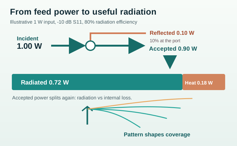
Follow the power in the figure: some reflects at the port, some becomes heat, and the remainder radiates in different directions.

• Directivity: how strongly the pattern concentrates power compared with an isotropic reference.
• Gain: directivity with radiation efficiency included.
• Realized gain: gain with feed mismatch included as well.
• Practical check: a data sheet must say which gain it reports.

Quantity	Physical meaning	When it matters
$S_{11}$ / return loss	How much incident feed power reflects back at the port	Checking matching over the operating band
Radiation efficiency	Radiated power divided by accepted power	Distinguishing a lossy antenna from a useful radiator
Realized gain	Directional gain after mismatch loss	Comparing installed link-budget inputs on a consistent basis
Radiation pattern and HPBW	Where energy goes and the main-lobe half-power width	Planning coverage, pointing, and interference
Polarization	Orientation or trajectory of the electric field	Matching Tx/Rx antennas and interpreting cross-polarized ports

• $|S_{11}|^2$: reflected power fraction for the stated one-port reference impedance.
• Why matching is not enough: a matched resistor can absorb power without radiating it.

For a reference impedance $Z_0$ and antenna input impedance $Z_{\mathrm{in}}$, the reflection coefficient is

$$\Gamma=\frac{Z_{\mathrm{in}}-Z_0}{Z_{\mathrm{in}}+Z_0}, \qquad S_{11,\mathrm{dB}}=20\log_{10}|\Gamma|$$

• $\Gamma$: feed-port reflection coefficient; $|\Gamma|^2$ is the reflected power fraction.
• $Z_{\mathrm{in}}$: antenna input impedance; $Z_0$: stated reference impedance.
• $S_{11,\mathrm{dB}}$: reflection expressed in dB, assuming the same reference.

The accepted and radiated powers can then be separated:

$$P_{\mathrm{accepted}}=P_{\mathrm{incident}}(1-|\Gamma|^2), \qquad P_{\mathrm{radiated}}=\eta_{\mathrm{rad}}P_{\mathrm{accepted}}$$

• $P_{\mathrm{incident}}$, $P_{\mathrm{accepted}}$, $P_{\mathrm{radiated}}$: power reaching the port, entering the antenna, and actually radiated.
• $\Gamma$: feed-port reflection coefficient from the preceding equation.
• $\eta_{\mathrm{rad}}$: radiation efficiency, between 0 and 1.

References for this section3

• C. A. Balanis, Antenna Theory: Analysis and Design, 4th ed., Wiley.
• MathWorks, Antenna Toolbox User's Guide: directivity, gain, realized gain, and EIRP.
• NIST, Antenna Gain and Polarization Calibration.

S-Parameters: Follow the RF Waves

Scattering parameters describe what happens to RF waves at the ports of a device. They are complex values, so both magnitude and phase can be measured over frequency.

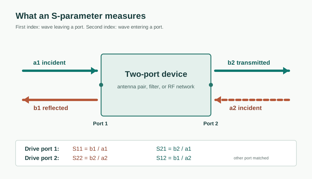
• Port: a defined RF connection or antenna feed with a reference impedance, commonly but not necessarily $50\ \Omega$.
• Incident wave $a_i$: the wave entering port $i$.
• Outgoing wave $b_i$: the wave leaving port $i$.
• Index rule: in $S_{ij}$, $j$ is the excited input port and $i$ is the observed output port.

For a two-port network:

$$\begin{bmatrix}b_1\\b_2\end{bmatrix} =\begin{bmatrix}S_{11}&S_{12}\\S_{21}&S_{22}\end{bmatrix} \begin{bmatrix}a_1\\a_2\end{bmatrix}$$

• $a_1,a_2$: incident waves at ports 1 and 2; $b_1,b_2$: outgoing waves.

• $S_{11}$: reflection back into port 1 when port 2 is matched.

• $S_{22}$: reflection back into port 2 when port 1 is matched.

• $S_{21}$: forward transfer from port 1 to 2; $S_{12}$: reverse transfer from port 2 to 1.

• One antenna port: $S_{11}$ checks feed matching, not radiation efficiency.

• Two antenna ports: $S_{21}$ or $S_{12}$ indicate coupling under stated terminations; neither alone proves independent MIMO channels.

References for this section3

• C. A. Balanis, Antenna Theory: Analysis and Design, 4th ed., Wiley.
• Rohde & Schwarz, Understanding S-parameters.
• NIST, Antenna Gain and Polarization Calibration.

Return Loss, Mismatch, and VSWR

Three views of the same one-port reflection are useful:

$$P_{\mathrm{reflected}}/P_{\mathrm{incident}}=|S_{11}|^2, \qquad RL=-20\log_{10}|S_{11}|$$

• $P_{\mathrm{reflected}}/P_{\mathrm{incident}}$: reflected power fraction at the stated port reference.
• $S_{11}$: complex reflection coefficient for this one-port measurement; $|S_{11}|$ is its wave-amplitude ratio.
• $RL$: positive return loss in dB. By contrast, $S_{11,\mathrm{dB}}=20\log_{10}|S_{11}|$ is usually negative; $RL=-S_{11,\mathrm{dB}}$.

$$\mathrm{VSWR}=\frac{1+|S_{11}|}{1-|S_{11}|}$$

• $\mathrm{VSWR}$: voltage standing-wave ratio on a line referenced to the same impedance.
• $|S_{11}|$: reflection magnitude, from 0 (perfect match) toward 1 (complete reflection).

Example: $S_{11}=-10$ dB means $|S_{11}|\approx0.316$, about 10% reflected power, 90% accepted power, $RL=10$ dB, and VSWR about 1.92. This does not mean 90% radiates: internal loss must still be checked.

References for this section3

• Keysight, Network Analyzer Basics: return loss and VSWR.
• C. A. Balanis, Antenna Theory: Analysis and Design, 4th ed., Wiley.
• NIST, Measuring Antennas Above 1 GHz.

Transmission and Isolation

$$S_{21}=\left.\frac{b_2}{a_1}\right|_{a_2=0}, \qquad S_{12}=\left.\frac{b_1}{a_2}\right|_{a_1=0}$$

• $S_{21}$: complex forward wave ratio with port 2 matched.
• $S_{12}$: complex reverse wave ratio with port 1 matched.
• $a_i,b_i$: incident and outgoing waves shown in the diagram; the zero subscript condition means the other port has no incident wave from its matched termination.
• For a passive two-port device: $20\log_{10}|S_{21}|$ reports transfer in dB; a more negative number can mean more insertion loss.
• For antenna ports: a more negative coupling value can indicate better port isolation, but pattern, efficiency, correlation, and over-the-air channel still matter.

Under matched, equal-reference port conditions, a useful positive loss convention is:

$$IL_{21}=-20\log_{10}|S_{21}|, \qquad I_{21}=-20\log_{10}|S_{21}|$$

• $IL_{21}$: insertion loss in dB when port 2 is the intended output of a passive path.
• $I_{21}$: isolation in dB when transfer from port 1 to port 2 is unwanted coupling.
• $|S_{21}|$: forward wave-amplitude ratio with the other port matched; the arithmetic is the same, but the engineering question differs.
• Example: $S_{21}=-20$ dB corresponds to about 1% transferred power under these matched-reference conditions, or 20 dB isolation between ports.

Measurement order: calibrate the vector network analyser at the chosen reference plane, state port impedance and cable/de-embedding treatment, sweep the intended band, then compare $S$-parameters at the same frequency and setup.

References for this section3

• C. A. Balanis, Antenna Theory: Analysis and Design, 4th ed., Wiley.
• NIST, Antenna Gain and Polarization Calibration.
• MathWorks, Antenna Toolbox User's Guide: directivity, gain, realized gain, and EIRP.

Worked Example: Matching Is Not Efficiency

Suppose 1 W is incident on an antenna with $S_{11}=-10$ dB and radiation efficiency of 80%:

1. At the port: $|S_{11}|^2=0.1$; 0.1 W reflects and 0.9 W is accepted.
2. Inside the antenna: $0.8\times0.9=0.72$ W is radiated; 0.18 W is lost internally.
3. In the useful direction: if directivity is 12 dBi, gain is $12+10\log_{10}(0.8)\approx11.0$ dBi. Including mismatch gives realized gain of about 10.6 dBi.

A second antenna with the same matching could radiate less if its efficiency is lower. These values assume efficiency and directivity at the same frequency and direction.

References for this section3

• C. A. Balanis, Antenna Theory: Analysis and Design, 4th ed., Wiley.
• MathWorks, Antenna Toolbox User's Guide: directivity, gain, realized gain, and EIRP.
• NIST, Antenna Gain and Polarization Calibration.

Radiation Pattern and Beamwidth

Radiation pattern shows how radiated strength changes with direction. It may be a power/intensity pattern or a field-amplitude pattern; check the plotted quantity and normalization.

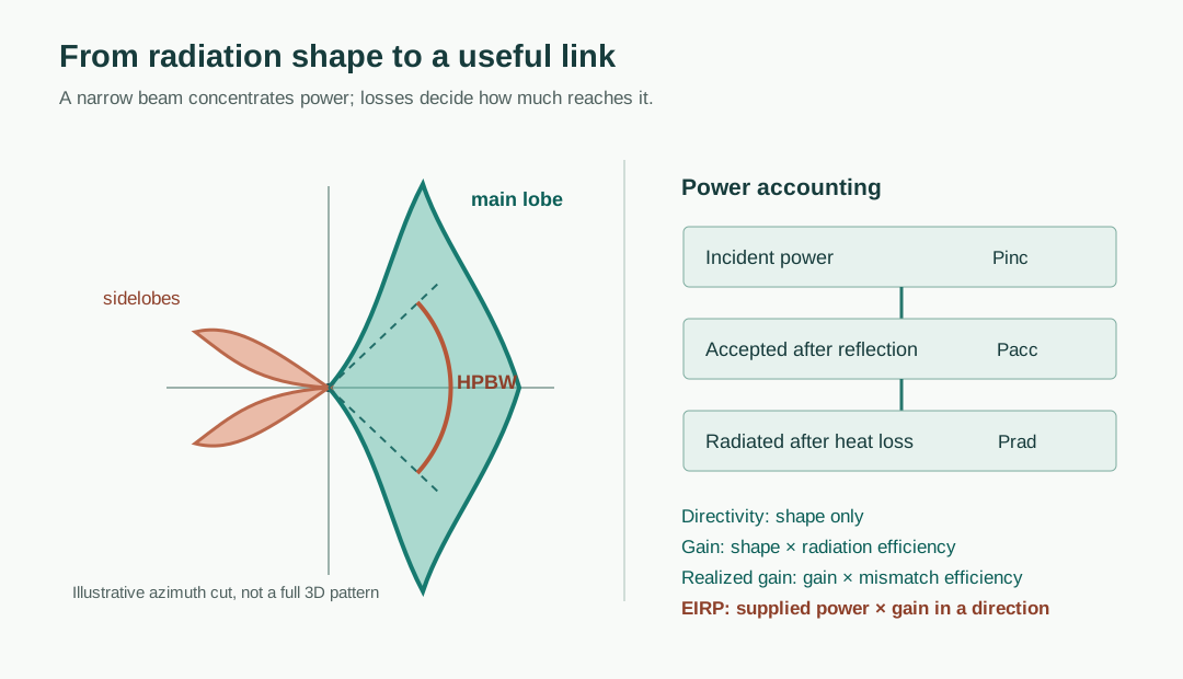
• Main lobe: strongest radiation direction; a narrower lobe often raises peak gain but covers less angle.
• Sidelobes: smaller peaks that can illuminate unintended users or interferers.
• Back radiation: power sent behind the intended direction.
• Read a pattern with: frequency, polarization, cut plane, and normalization. An azimuth slice is not the full 3D pattern.

Half-power beamwidth (HPBW) measures the angle between the two main-lobe directions at half the peak power:

$$U(\theta_1,\phi_0)=U(\theta_2,\phi_0)=\frac{U_{\max}}{2}, \qquad \mathrm{HPBW}=|\theta_2-\theta_1|$$

• $U(\theta,\phi)$: radiation intensity in direction $(\theta,\phi)$, in W/sr.
• $U_{\max}$: peak intensity on the stated cut; $\phi_0$: fixed plane of that cut.
• $\theta_1,\theta_2$: the two half-power angles around the main lobe.
• $\mathrm{HPBW}$: angular width, usually in degrees. Half power is $-3.01$ dB relative to peak.

References for this section3

• C. A. Balanis, Antenna Theory: Analysis and Design, 4th ed., Wiley.
• NIST, Antenna Gain and Polarization Calibration.
• MathWorks, Antenna Toolbox User's Guide: directivity, gain, realized gain, and EIRP.

Directivity, Gain, and EIRP

Radiation intensity turns the far-field power density at a range into a direction-dependent power per solid angle:

$$U(\theta,\phi)=r^2S_{\mathrm{rad}}(r,\theta,\phi), \qquad P_{\mathrm{rad}}=\int_{4\pi}U(\theta,\phi)\,d\Omega$$

• $U(\theta,\phi)$: radiation intensity in W/sr at direction $(\theta,\phi)$.
• $S_{\mathrm{rad}}$: far-field power density in W/m² at distance $r$ in metres.
• $P_{\mathrm{rad}}$: total power radiated over all directions, in watts.
• $d\Omega$: small solid angle in steradians; $4\pi$ denotes the entire sphere.

Directivity compares one direction with an ideal isotropic radiator that radiates the same total power:

$$D(\theta,\phi)=\frac{4\pi U(\theta,\phi)}{P_{\mathrm{rad}}}$$

• $D(\theta,\phi)$: dimensionless directional concentration; $10\log_{10}D$ gives dBi.
• $U(\theta,\phi)$: radiation intensity in that direction.
• $P_{\mathrm{rad}}$: total radiated power; $4\pi$ is the full-sphere solid angle in sr.
• Physical point: directivity describes shape, not conductor/dielectric loss or feed mismatch.

Radiation efficiency and gain include the antenna's internal loss:

$$\eta_{\mathrm{rad}}=\frac{P_{\mathrm{rad}}}{P_{\mathrm{accepted}}}, \qquad G(\theta,\phi)=\eta_{\mathrm{rad}}D(\theta,\phi)$$

• $\eta_{\mathrm{rad}}$: fraction of accepted power radiated, between 0 and 1.
• $P_{\mathrm{accepted}}$: power entering the antenna after feed reflection.
• $P_{\mathrm{rad}}$: power actually radiated; $D$: directivity; $G$: directional power gain relative to isotropic.
• In dB: $G_{\mathrm{dBi}}=D_{\mathrm{dBi}}+10\log_{10}\eta_{\mathrm{rad}}$.

Realized gain also includes mismatch at the stated feed:

$$G_{\mathrm{realized}}(\theta,\phi)=(1-|S_{11}|^2)G(\theta,\phi)$$

• $G_{\mathrm{realized}}$: gain including feed mismatch, for this single-port reference.
• $|S_{11}|^2$: reflected power fraction; $1-|S_{11}|^2$ is accepted power fraction.
• $G$: gain after internal radiation loss but before mismatch loss.

EIRP is the isotropic power that would produce the same far-field strength in a chosen direction:

$$\mathrm{EIRP}_{\mathrm{dBm}}(\theta,\phi)=P_{\mathrm{tx,dBm}}-L_{\mathrm{feed,dB}}+G_{\mathrm{dBi}}(\theta,\phi)$$

• $P_{\mathrm{tx,dBm}}$: power at the point before the stated feed loss.
• $L_{\mathrm{feed,dB}}$: loss between that point and the antenna's accepted-power reference.
• $G_{\mathrm{dBi}}(\theta,\phi)$: directional gain at the antenna input in dBi.
• $\mathrm{EIRP}_{\mathrm{dBm}}$: equivalent isotropic radiated power in that direction. If using realized gain at an incident-port reference, do not subtract mismatch again.

Worked comparison: take 1 W (30 dBm) at the incident port, 12 dBi directivity, 80% radiation efficiency, and $S_{11}=-10$ dB.

1. Gain: about 11.0 dBi after radiation loss.
2. Realized gain: about 10.6 dBi after reflection at the feed.
3. Peak EIRP: about 40.6 dBm from this incident-port reference.

References for this section3

• MathWorks, Antenna Toolbox User's Guide: directivity, gain, realized gain, and EIRP.
• C. A. Balanis, Antenna Theory: Analysis and Design, 4th ed., Wiley.
• NIST, Antenna Gain and Polarization Calibration.

What a Pattern Can and Cannot Say

Polarization mismatch means the transmitting and receiving electric-field orientations do not line up, even when their beams do.

$$\eta_{\mathrm{pol}}=\cos^2\psi$$

• $\eta_{\mathrm{pol}}$: ideal linear-polarization power-coupling fraction.

• $\psi$: angle between the two linear polarizations.

• $45^\circ$ mismatch: half the ideal power couples, a 3 dB loss.

• $90^\circ$ mismatch: zero coupling in the ideal linear model.

• Link lesson: matching and peak gain do not fix wrong pointing or polarization.

References for this section3

• C. A. Balanis, Antenna Theory: Analysis and Design, 4th ed., Wiley.
• NIST, Antenna Gain and Polarization Calibration.
• MathWorks, Antenna Toolbox User's Guide: directivity, gain, realized gain, and EIRP.

Gain, Aperture, and Beamwidth

• Peak gain: concentration of existing radiation, not extra generated power.

• Electrical aperture: antenna size measured relative to wavelength; a larger one can usually make a narrower beam.

• HPBW: angle between the two main-lobe directions at half peak power ($-3$ dB).

• Coverage check: report azimuth and elevation cuts; a beam can be narrow in one plane and broad in the other.

• Data sheet: inspect patterns across the band, not only one peak dBi number.

• Sidelobes/back radiation: check unintended illumination and interference.

• Array: element pattern and array factor combine; element gain alone cannot predict the steered beam.

References for this section3

• C. A. Balanis, Antenna Theory: Analysis and Design, 4th ed., Wiley.
• NIST, Antenna Gain and Polarization Calibration.
• MathWorks, Antenna Toolbox User's Guide: directivity, gain, realized gain, and EIRP.

Where This Is Used

• Coverage planning: select a pattern and downtilt that illuminate the intended area.

• Link budgets: use the appropriate directional gain, feed loss, and pointing loss.

• MIMO and arrays: inspect port isolation and correlation as well as the element pattern.

• Measurement: check $S_{11}$ with a calibrated network analyser, then measure radiation pattern and gain with an appropriate antenna setup; one test does not replace the other.

• Rooftop sector: pattern and downtilt decide whether power reaches the street or overshoots it.

• Point-to-point backhaul: a narrow beam adds directional gain but requires precise alignment.

• Handset: efficiency and hand detuning can matter more than laboratory peak gain.

• Dual-polarized MIMO: cross-polar discrimination and port isolation join gain and pattern checks.

Practical checklist:

1. State the band and reference impedance; plot $S_{11}$ across the band.
2. Measure efficiency and realized gain; inspect co- and cross-polar patterns.
3. Repeat at representative steering angles or installation positions.
4. Judge values against the required link margin and coverage region.

• Visual follow-up: gain, beamwidth, polarization, and evolution.
• Next physical step: propagation fundamentals.

References for this section3

• C. A. Balanis, Antenna Theory: Analysis and Design, 4th ed., Wiley.
• NIST, Antenna Gain and Polarization Calibration.
• MathWorks, Antenna Toolbox User's Guide: directivity, gain, realized gain, and EIRP.